


In the last post I argued that training at scale is a systems problem, and the system you’re working against is the bandwidth hierarchy of your physical cluster. Each parallelism paradigm is a bet about where in that hierarchy you can afford to communicate.
This post answers the next question: what bets can you actually make?
When you read the literature, the answer looks complicated. DDP, ZeRO-1, ZeRO-2, ZeRO-3, FSDP, HSDP, TP, SP, PP (GPipe, 1F1B, interleaved, zero-bubble), CP, EP, ring attention, expert choice, DeepEP - every framework has its own vocabulary, every paper introduces a new acronym, and a new practitioner could be forgiven for thinking there are dozens of distinct techniques to learn.
The reality is simpler. A training step has a small number of dimensions you can split work along, and every named paradigm is a strategy for splitting one of those dimensions: sometimes one alone, sometimes a few combined. Once you have the dimensions in your head, the zoo of paradigms organizes itself into a small map.
The table below is the map at a glance - what each axis splits, what communication it forces, which tier of fabric it lives on. If you’ve worked with a few of these and just need the layout, the table is the post. If you want to know why each row reads the way it does, the sections after it walk through each axis in turn.
Modifiers - knobs within an axis, not separate axes:
There are five dimensions worth knowing. Here they are, in the order I find easiest to remember.
1. Batch (B): data parallelism
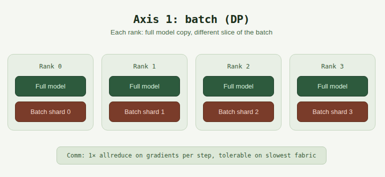
What gets split: the batch of training examples. Each rank processes a different shard of the batch through the same model weights.
Communication primitive: AllReduce on gradients at the end of each step. Each rank computes a gradient on its data shard; the cluster sums them so every rank ends up with the same averaged gradient.
Paradigm names: DDP (the textbook version), and all the ZeRO/FSDP/HSDP variants which we’ll discuss separately because they’re really refinements of DP rather than a new axis.
Why this exists: it’s the trivial parallelism - you can always train on more data in parallel. The forcing function is that one GPU’s batch is too small to get statistically meaningful gradients in reasonable time.
Cost: one allreduce per step on the full gradient (~2P bytes per rank). This is the cheapest communication pattern in the menu because it’s infrequent (once per step, not once per layer) and can be overlapped with backward compute. It’s the bottom of the communication intensity hierarchy.
Where it sits: tolerable on the slowest fabric in your hierarchy (inter-rack IB). This is why DP is the outermost layer of most composition recipes - it can pay the slowest fabric without bleeding throughput.
2. Hidden dimension (H): tensor parallelism
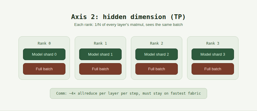
What gets split: the matmul itself. Each linear layer’s weight matrix is sharded, column-wise for some layers, row-wise for others, and the matmul is distributed across ranks accordingly.
Communication primitive: AllReduce inside each layer. The classic Megatron-LM recipe gets you down to one allreduce per attention block and one per MLP block, so roughly two allreduces per layer per microbatch per pass, or four per layer per step counting backward.
Paradigm names: TP (Megatron-style).
A note on naming before we go further. There’s a related technique called Sequence Parallelism (SP) which is the standard companion to TP. SP shards the activations of layernorm and dropout, the elementwise operations that sit between TP’s matmul regions, along the sequence dimension. It’s a free trick: AllReduce = ReduceScatter + AllGather , so SP turns TP’s region-boundary all-reduces into a reduce-scatter and all-gather pair that moves the same total bytes but leaves activations sharded between regions instead of replicated. The result is the same activation memory savings TP gives you for matmul tensors, now extended to the non-matmul stuff.
The naming is unfortunate. “Sequence parallelism” sounds like the general technique for sharding the sequence dimension, but in current usage (matching Megatron-Core, Transformer Engine, and most frontier framework documentation), SP specifically means this TP companion - sharding only the elementwise activations between TP regions, not the attention computation itself. The general technique for sharding sequence across attention is a different thing called Context Parallelism (CP), which gets its own section below. Some papers from 2022-2023 use “sequence parallelism” loosely to mean either. This series uses SP narrowly (the TP companion) and CP for the broader attention-sharding story.
So: SP rides with TP everywhere TP appears. It’s not a separate axis; it’s how you should always run TP at scale.
Why this exists: when a single layer’s parameters or activations don’t fit on one GPU. Also useful when activation memory dominates at long context, even if the model would otherwise fit.
Cost: many allreduces per layer, on the critical path of compute (the next operation can’t start until the allreduce completes). With ~80 layers and 4 allreduces per layer, that’s 320 hard sync points per step. Even small, this adds up - TP communication is often 10-30% of step time at typical TP=8.
Where it sits: the top of the bandwidth hierarchy. TP must stay within the fast intra-node domain (NVLink/NVSwitch: 8 GPUs on H100, 72 on GB200 NVL72). Push it across InfiniBand and your MFU collapses, because the chattiest workload now lives on the slowest fabric.
3. Layer depth (L): pipeline parallelism
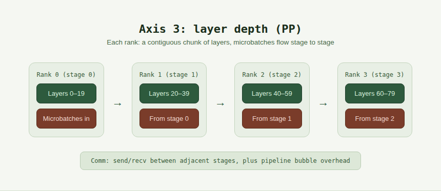
What gets split: the model’s layers. Each rank (or rank group) owns a contiguous chunk of layers - the “pipeline stage.” Forward activations flow from stage 0 → 1 → 2 → ...; gradients flow back the other way.
Communication primitive: point-to-point send/recv between adjacent stages. One activation tensor goes forward; one gradient tensor comes back. Not collectives.
Paradigm names: PP, GPipe, PipeDream, 1F1B, interleaved 1F1B, zero-bubble PP. The progression in the literature is mostly about scheduling: how to fill the pipeline to minimize the idle “bubble” while keeping activation memory bounded.
Why this exists: when even TP + FSDP can’t fit the model on the fast fabric. PP lets you spread the model across many nodes by giving each node a stage instead of a sharded copy.
Cost: two related costs. First, the pipeline bubble - idle time on each stage while microbatches propagate. Bubble fraction is roughly (N-1)/(M+N-1) for N stages and M microbatches, so M has to be much larger than N to keep the bubble small. Second, stashed activations: each stage holds onto activations for in-flight microbatches until their backward pass arrives. The send/recv communication itself is cheap; the scheduling complexity is what makes PP hard.
Where it sits: tolerable on InfiniBand. The messages are large but infrequent (per stage boundary, not per layer), and PP doesn’t depend on a fully-connected fast domain. This is why PP is typically the “across nodes” layer in composition recipes.
4. Sequence - attention (S): context parallelism
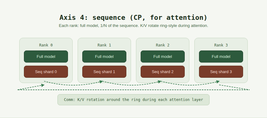
What gets split: the sequence dimension across the attention computation itself. Each rank persistently holds 1/N of the sequence’s Q, K, V. To make attention work (every Q must see every K), K and V chunks rotate around the ranks while attention is computed in pieces.
Communication primitive: ring rotation of K/V shards between adjacent ranks (point-to-point send/recv, but in a ring pattern). Combined with the online-softmax trick (the same algorithmic identity FlashAttention uses) to combine partial attention results without ever materializing the full attention matrix.
Paradigm names: CP, Ring Attention, Striped Attention (a load-balanced variant for causal masking).
Why this exists: at long context (typically 16K+ tokens), the attention activation memory becomes the dominant cost, and you can’t reduce it further with TP alone (head sharding caps out at the number of heads, and activations per head are quadratic in sequence).
Cost: N-1 ring rotations per attention layer, where N is the CP degree. The cost is high enough that CP only pays for itself past ~16K-32K sequence on H100 — below that, the rotation communication exceeds the memory savings. On GB200 NVL72 the crossover shifts down to maybe 4K-8K because the ring runs on much faster fabric.
Where it sits: middle of the hierarchy. CP wants fast fabric (the ring rotation is on the critical path of attention), but tolerates inter-node IB at long context where the per-chunk attention compute is large enough to hide the rotation. Typically composed alongside TP.
5. Experts (E): expert parallelism
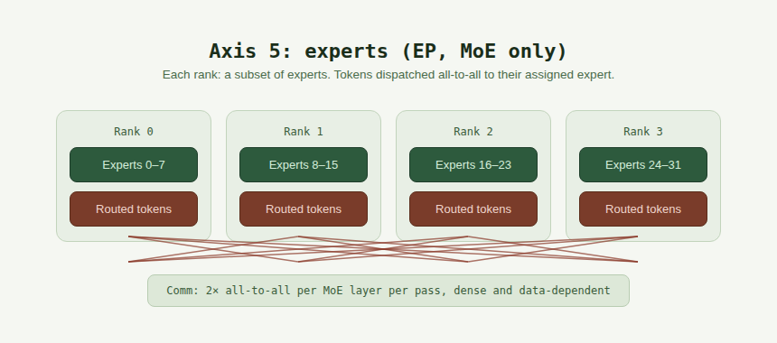
What gets split: experts in a Mixture-of-Experts model. Each rank holds and computes for only its assigned subset of experts.
Communication primitive: all-to-all. Twice per MoE layer per forward pass - once to dispatch tokens to the ranks holding their assigned experts, once to combine the expert outputs back to the originating ranks.
Paradigm names: EP, expert sharding. The choice of routing algorithm (top-k, expert choice, auxiliary-loss-free) shapes the load distribution but doesn’t change the basic communication pattern.
Why this exists: MoE models decouple parameter count from compute per token. A 1T-parameter MoE might activate only 37B parameters per token. Those 1T parameters still have to live somewhere; distributing them across DP ranks wastes memory (every rank holds all experts but uses few). EP makes each rank specialize.
Cost: all-to-all is the densest communication pattern in this menu. Every rank sends data to every other rank, in both directions, simultaneously. The traffic is also uneven across steps - if the router sends 30% of tokens to one expert, that expert’s rank receives 30% of all traffic. Load imbalance directly compounds the communication cost. At frontier scale, EP all-to-all can be the single largest component of step time and motivates custom kernels (DeepSeek’s DeepEP).
Where it sits: wants fast moderate-distance fabric. Within a single fast domain is ideal (EP=64 within a GB200 NVL72 rack is a meaningful sweet spot). Across nodes via IB works but requires careful tuning of both the routing (to balance load) and the communication kernels (to handle the dense traffic).
The modifiers: SP and FSDP
Two more names you’ll encounter in the literature deserve a callout, because the field talks about them as if they’re peer techniques to TP/PP/CP/EP and they aren’t.
SP is the TP companion described in section 2. It’s not a separate axis: it’s how you should always run TP at scale. The reason it gets its own name is historical (Megatron published it as a distinct paper) and the reason it stuck is that you can run TP without SP, badly. But conceptually, SP is part of TP. Anywhere this series talks about TP, assume SP rides along.
FSDP is a refinement of DP. DDP replicates the entire model state on every DP rank. ZeRO-1 shards optimizer states across DP ranks. ZeRO-2 also shards gradients. ZeRO-3 (= FSDP) also shards parameters. Each level reclaims memory DDP was wasting on redundant copies, at additional communication cost.
The right way to think about it: DP is an axis (the batch dimension). FSDP is a choice about how aggressively to shard state along that same axis. HSDP is “FSDP within one node, DDP across nodes”: same axis, hierarchical sharding policy. The DDP-vs-FSDP-vs-HSDP choice is a within-axis knob, not a new axis. The dedicated DP post will go deep on which knob to pick when.
The map of “things you can adjust”: five axes, plus a sharding-aggressiveness knob within DP, plus the TP-with-or-without-SP knob (always: with).
The composition preview
When you hear “3D parallelism” or “5D parallelism,” that’s just picking multiple axes at once. A typical frontier dense recipe (Llama 3 style) uses three axes: TP × PP × DP. A long-context recipe might add CP for four. A frontier MoE recipe might use TP × EP × PP × DP for four, with EP replacing some of what TP normally does.
The geometry of the cluster sets the constraints: TP wants the fast fabric, so it goes intra-node. PP tolerates IB, so it goes across nodes. DP tolerates the slowest fabric, so it’s the outermost layer. CP and EP fit in the middle, with placement details that depend on the specific cluster topology.
The next several posts will take each axis seriously, one at a time. We’ll see how each one’s communication primitive maps to bandwidth and latency budgets, where it breaks under load, what knobs frameworks expose, and what surprises you when you scale it up. Then we’ll come back to composition - by that point, “4D parallelism” should feel less like jargon and more like an obvious consequence of picking the right axis for each tier of your machine.
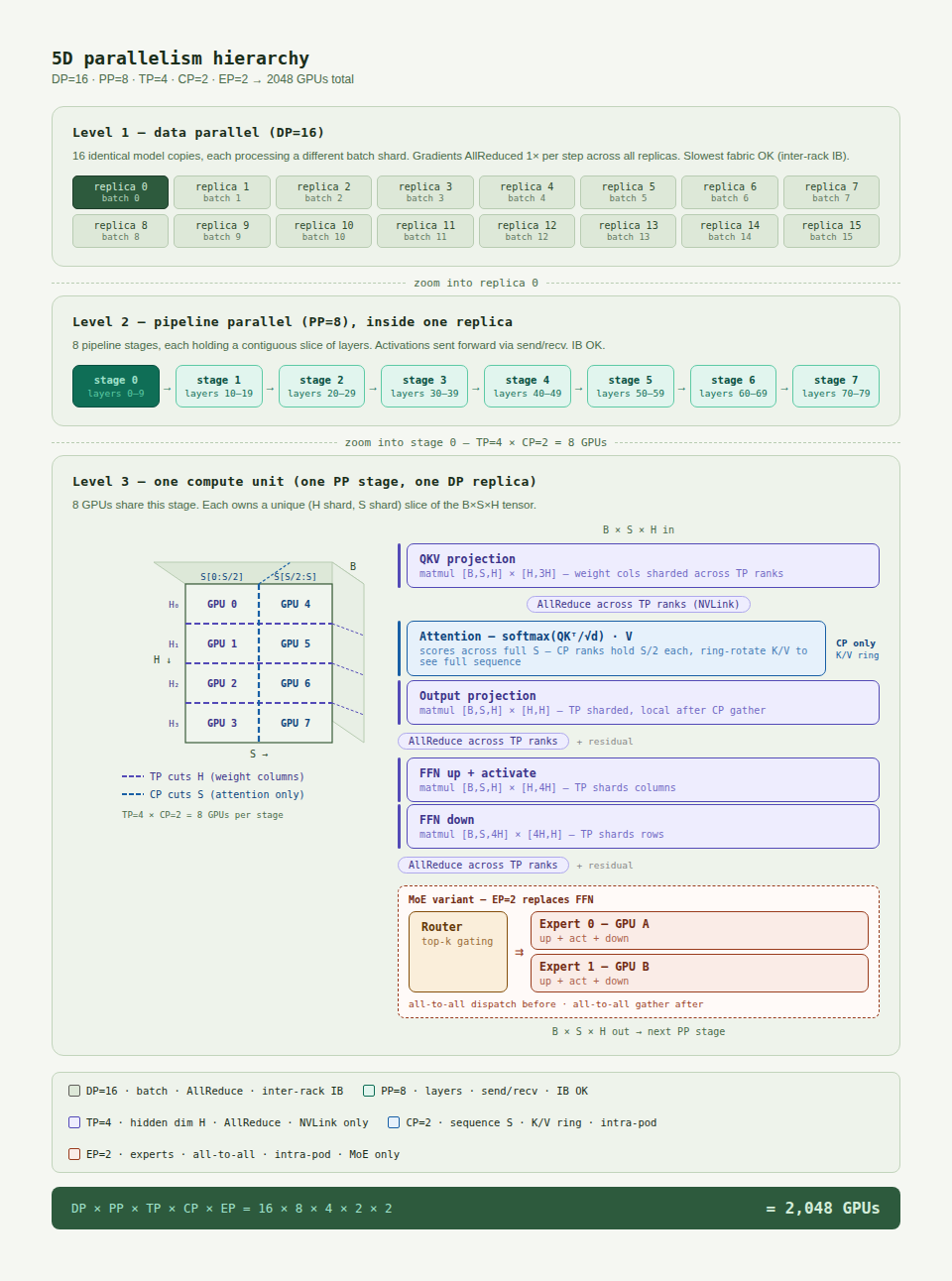
Before the takeaway, it's worth pausing on what 5D composition actually looks like end-to-end. The diagram below zooms three times: from the cluster (DP across 16 replicas), into one replica (PP across 8 stages), into one stage (TP × CP × optional EP across 8 GPUs), all the way down to where a single QKV projection happens. It's the picture I keep coming back to, because it makes the nesting obvious in a way prose can't: each axis isn't a separate technique you bolt on, it's a level of zoom on the same physical cluster.
The takeaway
If I could put one thing in your head before the next post: There are five dimensions you can split work along, and the right composition is the one where each axis lives at the right level of zoom. Every paradigm name you've heard is a strategy for one of them, or a combination. Pick the dimensions by asking what your bottleneck is; pick the degree by asking what tier of your fabric you can afford to communicate.
Once you have this map, the rest of the series is a tour of each axis in turn.
Next post: data parallelism in depth: what DDP actually does, why bucketing exists, where it breaks at scale, and how ZeRO-2 recovers most of the wasted memory essentially for free.